Aligning protein-generative models to experimental fitness with ProteinDPO

Generative model alignment

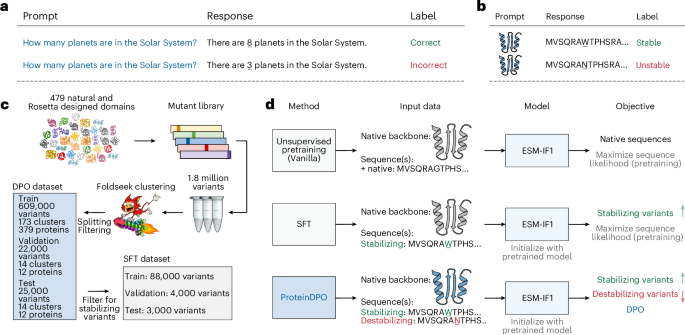
Generative AI applications are now routinely fine-tuned with feedback-based RL during post-training, which has been crucial for the success of applications in the natural language domain^49,50. Here, we provide a brief overview of the classical model training pipeline, which consists of three stages: SFT, feedback collection and RL fine-tuning^51,52.

SFT

Here, we define SFT as continuing the original pretraining objective on high-quality samples from a downstream labeled dataset. In this work for example, for SFT on the ‘Megascale’ dataset, high-quality samples are sequences which achieve superior stability to the native sequence. During the SFT stage we use a dataset of input-output pairs, \({\mathcal{D}}={\{{\bf{x}},{\bf{y}}\}}_{i = 1}^{N}\) and train a model p_θ with next-token maximum likelihood loss on high-quality pairs, where y_i is the ith token of the output y

Feedback stage

During the feedback stage we use the base model or the SFT model p_SFT and a set of inputs to sample a number K > 0 of candidate completions y⁽ⁱ⁾, …, y^(K) per prompt x from a dataset of preferences \({{\mathcal{D}}}_{{\rm{pref}}}\). Feedback can be provided in several ways:

1. (1)

   Prior RLHF work has used ranking type of comparisons in which the candidate outputs are ranked \({{\bf{y}}}^{({i}_{1})}\succ {{\bf{y}}}^{({i}_{2})}\succ \ldots \succ {{\bf{y}}}^{({i}_{K})}\), with pairwise rankings being a popular choice. To use this data from the RL stage, we need to extract an evaluation score from it. We usually assume a parameterization of the preference distribution, such as the Plackett-Luce^53,54 choice model (or the Bradley–Terry⁵⁵ for pairwise data). In the most general case, given the permutation \(\tau :{{\bf{y}}}^{(1)},\ldots ,{{\bf{y}}}^{(K)}\to {{\bf{y}}}^{({i}_{1})},\ldots ,{{\bf{y}}}^{({i}_{k})}\), we have

   $$P(\tau | {{\bf{y}}}^{(1)},\ldots ,{{\bf{y}}}^{(K)},{\bf{x}})=\prod _{k=1}^{K}\frac{\exp (r({\bf{x}},{{\bf{y}}}^{({i}_{k})}))}{{\sum }_{j=k}^{K}\exp (r({\bf{x}},{{\bf{y}}}^{({i}_{\!j})}))}.$$

   (2)

   We can then form ulate this as a maximum likelihood loss over the reward model

   $${{{ \mathcal L }}}_{r}=-{{\mathbb{E}}}_{{\bf{x}},{{\bf{y}}}^{({i}_{1})},\ldots ,{{\bf{y}}}^{({i}_{K})}\sim {{{ \mathcal D }}}_{\mathrm{pref}}}\sum _{k=1}^{K}\left[r\left({\bf{x}},{{\bf{y}}}^{({i}_{k})}\right)-{\mathrm{log}}\sum _{j=k}^{K}\exp \left(r\left({\bf{x}},{{\bf{y}}}^{({i}_{\!j})}\right)\right)\right].$$

   (3)

2. (2)

   In the case of pairwise rankings y^w ≻ y^l, this just reduces to the standard binary logistic regression loss,

   $${{{ \mathcal L }}}_{r}=-{{\mathbb{E}}}_{{\bf{x}},{{\bf{y}}}^{w},{{\bf{y}}}^{l}\sim {{{ \mathcal D }}}_{\mathrm{pref}}}\left[{\mathrm{log}}\sigma (r({\bf{x}},{{\bf{y}}}^{w})-r({\bf{x}},{{\bf{y}}}^{l}))\right],$$

   (4)

   where σ(⋅) is the sigmoid function. Notice that if we are provided with a complete ranking over K candidates then we can construct \(\left(\begin{array}{c}K\\ 2\end{array}\right)\) pairwise rankings, which was used in prior works²². These can still be easily optimized together since we still require a single forward pass through the reward model.

3. (3)

   Alternatively a numerical score, r_i (such as used in a Likert scale) could be provided per candidate input-output pair (x, y⁽ⁱ⁾).

RL stage

During the RL stage we use a reference model p_ref, sometimes initialized as p_SFT from the SFT stage, and optimize the following RL problem:

We want to optimize a model p_θ to maximize the score, while also maintaining a distribution close to the reference model. The second terms aims to keep the model close to the distribution, which was used to collect the feedback data and prevent out-of-distribution issues⁵⁶.

Optimization algorithms

Two main algorithms have emerged for the optimization of the objective in equation (5): (1) classical RL algorithms, such as PPO⁵⁷, which use on-policy rollouts from the model; and (2) direct alignment algorithms, such as DPO¹⁶, which train fully-offline using only feedback data. Although successful in large scale-systems, such as GPT-4, the PPO pipeline requires a very accurate score model that can be queried in a continuous manner. Prior work has directly trained a separate score network r_θ(x, y) using the feedback data with the objective in equation (4) and directly applied PPO to the problem in equation (5) using the trained score model. However, such a pipeline can be quite complex, unstable and computationally expensive^58,59. DPO¹⁶ is an alternative to this algorithmic pipeline, which we present below.

DPO

The DPO algorithm is based on the observation that the objective in equation (5) has a closed form solution of the type

where

is an intractable partition function. The key insight of the DPO algorithm is the model-reward equivalency, that is,

Now, if instead of training a score model r_θ, we directly parameterize the generative model p_θ, we can use the preference data to directly optimize p_θ, essentially marginalizing the RL loop.

For the ranked objective, if we substitute the above expression into the Plackett–Luce reward model in equation (3), we obtain the following objective:

For the paired objective, If we instead use the pairwise objective in equation (4), we obtain the canonical form of the DPO objective

Here, due to the homogeneity of both the Plackett–Luce and Bradley–Terry model (that is, comparing several options for the same context), the untractable partition term Z(x) cancels out and we are left with tractable, fully offline objectives.

Weighted DPO algorithm

Prior methods, including DPO¹⁶, have all focused on extracting a per-sample score r(x, y) from rankings. However, if we have some external evaluation score, that is, data \({\{{\bf{x}},{{\bf{y}}}_{1},r({\bf{x}},{{\bf{y}}}_{1})\}}_{i=1}^{K}\), then this step is redundant. Given numerical scores, we could train a score model, using a regression-based framework and then use the standard PPO pipeline, but this approach inherits all the shortcomings of the standard RLHF pipeline. We could use the numerical scores to induce a ranking over candidates y_i and the apply the Plackett–Luce or Bradley–Terry DPO objectives in equations (9) and (10), respectively; however that faces two drawbacks:

1. 1.

   Plackett–Luce and Bradley–Terry both assume a particular parametric form of the ranking likelihood, that is, the rankings are inherently probabilistic, which would induce additional noise in the optimization procedure if we generate rankings based on those choice models.

2. 2.

   We can also generate rankings based on raw scores similarly to prior works⁶⁰. However, note that any monotone transformation would still induce the same relative rankings. That is, there might be actual relative information in the score which could be lost in such a scenario.

Weighted regression-based methods^61,62,63 are a good fit for this problem; however, they have been suboptimal in the large generative model setting and do not yield significant improvement⁶⁴. Instead, we will aim to develop a DPO type of algorithm that can efficiently utilize the numerical scores of the candidate sequences. Given an x and candidate sequences \({\{{{\bf{y}}}^{(i)},r({\bf{x}},{{\bf{y}}}^{(i)})\}}_{i = 1}^{K}\), consider the parameterized reward

That is a parameterized distribution p_θ(y∣x) induces a reward function r_θ(x, y), such that the model p_θ is the optimal solution for the corresponding RL problem in equation (5). Now, instead of aligning the generative model p_θ with some sampled rankings or preferences, we will instead minimize a distance function of the type D(r(x, y), r_θ(x, y)); that is, we will match the true score samples with the implicit ones. A remaining issue is that we still have the constraining partition function Z_θ(x) (because it depends on p_θ), which we would like to eliminate. When we consider

notice that the partition function Z_θ(x) was eliminated. In the same manner we have that

Notice now that w = (w⁽¹⁾, …, w^(K)) and \({{\bf{w}}}_{\theta }=({w}_{\theta }^{(1)},\ldots ,{w}_{\theta }^{(K)})\) are both valid probability distributions. In fact, the probability distributions resemble the Boltzmann distribution from statistical mechanics⁶⁵

where p(i) is the probability of the system being in a state i with energy E_i, and k_BT is the scaled absolute temperature of the system. Substituting r(x, y⁽ⁱ⁾) for the negative energy of the state −E_i, and considering k_BT, a parameter which allows us to scale the numerical scores r(x, y⁽ⁱ⁾), the weighted DPO objective is simply minimization of the Kullback–Leibler (KL) divergence \({{\mathbb{D}}}_{KL}[{\bf{w}}| {{\bf{w}}}_{\theta }]\) between the Boltzmann-like distributions parameterized by the generative model p_θ and numerical scores from the dataset \({\mathcal{D}}\). With some simple algebra, this yields:

In the case where we have only two candidate sequences y⁽¹⁾ and y⁽²⁾, this can be simplified to

That is, this is essentially a weighted version of the DPO algorithm. One interpretation is that this objective is the expected DPO objective under p(y⁽¹⁾ ≻ y⁽²⁾∣x) = w⁽¹⁾ and p(y⁽²⁾ ≻ y⁽¹⁾∣x) = w⁽²⁾. These objectives are theoretically optimal in the offline regime as they are both mode-seeking and use a ‘negative gradient’ formulation⁶⁴.

Implementation

Algorithm 1 Compute sequence log-likelihood

 1: Input: sequence y, encoded structure h

 2: Output: log-likelihood \(\log {p}_{\theta }({\bf{y}}| {\bf{h}})\)

 3: // Get logits via teacher forcing

 4: O ← TransformerDecoder(y_{[0: |y|−1]}, h) // Logits for next-token prediction

 5: // Convert logits to probabilities

 6: P ← Softmax(O) // Token probabilities over vocabulary

 7: // Compute log-likelihood as negative cross-entropy

 8: l ← − CrossEntropy(P, y_{[1: |y|]}) // Per-position negative loss

 9: \(\log {p}_{\theta }({\bf{y}}| {\bf{h}})\leftarrow {\sum }_{t}{\ell }_{t}\) // Sum over sequence positions

10: return \(\log {p}_{\theta }({\bf{y}}| {\bf{h}})\)

Algorithm 2 DPO for structure-conditioned protein language model (pairwise)

 1: Input: structure \({\bf{X}}\in {{\mathbb{R}}}^{L\times 3}\), preferred sequence y_w, dispreferred sequence y_l, reference log-likelihoods \(\log {p}_{{\rm{ref}}}({{\bf{y}}}_{w}| {\bf{X}})\) and \(\log {p}_{{\rm{ref}}}({{\bf{y}}}_{l}| {\bf{X}})\), KL penalty coefficient β

 2: Output: DPO loss \({{\mathscr{ \mathcal L }}}_{\mathrm{DPO}}\)

 3: // Encode structure once for both sequences

 4: h ← GVPEncoder(X)

 5: // Compute policy log-likelihoods for both sequences

 6: O_w, O_l ← TransformerDecoder(y_w, h), TransformerDecoder(y_l, h) // Logits

 7: \(\mathrm{log}{p}_{\theta }({{\bf{y}}}_{w}| {\bf{X}}),\mathrm{log}{p}_{\theta }({{\bf{y}}}_{l}| {\bf{X}})\leftarrow \,\mathrm{ComputeLogLikelihood}\,({{\bf{y}}}_{w},{{\bf{O}}}_{w}),\,\)\(\mathrm{ComputeLogLikelihood}\,({{\bf{y}}}_{l},{{\bf{O}}}_{l})\)

 8: // Compute pairwise DPO loss

 9: \({r}_{\theta }\leftarrow \log {p}_{\theta }({{\bf{y}}}_{w}| {\bf{X}})-\log {p}_{\theta }({{\bf{y}}}_{l}| {\bf{X}})\) // Policy log-ratio

10: \({r}_{\rm{ref}} \leftarrow {\rm{log}} \,\,{p}_{\rm{ref}} ({\bf{y}}_{w} |{\bf{X}}) – {\rm{log}}\,{p}_{\rm{ref}}({\bf{y}}_{l}|{\bf{X}})\) // Reference log-ratio

11: \({{{ \mathcal L }}}_{\mathrm{DPO}}\leftarrow -\mathrm{log}\sigma (\beta ({r}_{\theta }-{r}_{\mathrm{ref}}))\)

12: return \({{\mathcal{L}}}_{{\rm{DPO}}}\)

Algorithm 3 DPO for structure-conditioned protein language model (ranked)

 1: Input: structure \({\bf{X}}\in {{\mathbb{R}}}^{L\times 3}\), ranked sequences {y₁, …, y_K} where y₁ ≻ y₂ ≻ … ≻ y_K, reference log-likelihoods \({\{\log {p}_{{\rm{ref}}}({{\bf{y}}}_{k}| {\bf{X}})\}}_{k = 1}^{K}\), KL penalty coefficient β

 2: Output: DPO loss \({{\mathcal{L}}}_{{\rm{DPO}}}\)

 3: // Encode structure once for all sequences

 4: h ← GVPEncoder(X)

 5: // Compute policy log-likelihoods for all sequences

 6: for k = 1 to K do

 7:   O_k ← TransformerDecoder(y_k, h) // Logits

 8:  \(\log {p}_{\theta }({{\bf{y}}}_{k}| {\bf{X}})\leftarrow \,\text{ComputeLogLikelihood}\,({{\bf{y}}}_{k},{{\bf{O}}}_{k})\)

 9: end for

10: // Plackett–Luce ranking loss

11: \({{\mathcal{L}}}_{{\rm{DPO}}}\leftarrow 0\)

12: for k = 1 to K − 1 do

13:  \({r}_{k}\leftarrow {\beta}\,({\mathrm{log}}\,{p}_{\theta } ({{\bf{y}}}_{k}| {\bf{X}})- \mathrm{log}\,{p}_{\mathrm{ref}} ({{\bf{y}}}_{k}| {\bf{X}}))\) // Reward for rank k

14:  \({s}_{k}\leftarrow \log \mathop{\sum }\nolimits_{j = k+1}^{K}\exp \left(\beta (\log {p}_{\theta }({{\bf{y}}}_{j}| {\bf{X}})-\log {p}_{{\rm{ref}}}({{\bf{y}}}_{j}| {\bf{X}}))\right)\)

15:  \({{\mathscr{ \mathcal L }}}_{\mathrm{DPO}}\leftarrow {{\mathscr{ \mathcal L }}}_{\mathrm{DPO}}-\mathrm{log}\sigma ({r}_{k}-{s}_{k})\)

16: end for

17: return \({{\mathcal{L}}}_{{\rm{DPO}}}\)

Algorithm 4 DPO for structure-conditioned protein language model (weighted)

 1: Input: structure \({\bf{X}}\in {{\mathbb{R}}}^{L\times 3}\), sequences \({\{{{\bf{y}}}_{k}\}}_{k = 1}^{K}\), reference log-likelihoods \({\{\log {p}_{{\rm{ref}}}({{\bf{y}}}_{k}| {\bf{X}})\}}_{k = 1}^{K}\), preference targets \({\bf{w}}\in {{\mathbb{R}}}^{K}\), KL penalty coefficient β, temperature T

 2: Output: DPO loss \({{\mathcal{L}}}_{{\rm{DPO}}}\)

 3: // Encode structure once for all sequences

 4: h ← GVPEncoder(X)

 5: // Compute policy log-likelihoods for all sequences

 6: for k = 1 to K do

 7:   O_k ← TransformerDecoder(y_k, h) // Logits

 8:  \(\log {p}_{\theta }({{\bf{y}}}_{k}| {\bf{X}})\leftarrow \,\text{ComputeLogLikelihood}\,({{\bf{y}}}_{k},{{\bf{O}}}_{k})\)

 9: end for

10: // Compute reward-weighted cross-entropy loss

11: \({\bf{r}}\!\leftarrow\!\beta {\left[\log {p}_{\theta }({{\bf{y}}}_{1}| {\bf{X}})\!-\!\log {p}_{{\rm{ref}}}({{\bf{y}}}_{1}| {\bf{X}}),\!\ldots\! ,\log {p}_{\theta }({{\bf{y}}}_{K}| {\bf{X}})\!-\!\log {p}_{{\rm{ref}}}({{\bf{y}}}_{K}| {\bf{X}})\right]}^{\top }\)

12: \({{\mathcal{L}}}_{{\rm{DPO}}}\leftarrow -\mathop{\sum }\nolimits_{k = 1}^{K}{w}_{k}\log \frac{\exp ({r}_{k}/T)}{\mathop{\sum }\nolimits_{j = 1}^{K}\exp ({r}_{\!j}/T)}\) // Cross-entropy with temperature scaling

13: return \({{\mathcal{L}}}_{{\rm{DPO}}}\)

Datasets

Megascale

The Megascale dataset (v2 4/20/2023) served as the experimentally measured stability dataset from which we aligned the pretrained ESM-IF1. After filtering out data marked as unreliable for machine learning by Megascale authors, the dataset contained approximately 660,000 variants for 405 protein domains. The variants consisted of insertions, deletions, single and double substitutions. Similar to prior methods¹³, insertions and deletions were not considered as DPO training was designed to compare stabilities across the same structure; however, due to the robust nature of the model we were able to train and model with the double-mutations in the dataset. We additionally removed duplicate sequences. FoldSeek²³ clustering with the ‘easy-cluster algorithm was performed on all PDBs remaining in the Megascale dataset with an alignment threshold of 50%. From this, clusters were randomly assigned to respective train (90%), validation (5%) and test (5%) datasets to ensure generalizability of the model across different structures. Because the model is trained with sets of sequences for a common structure, either the ΔG (absolute) or ΔΔG (relative) of sequences were used for training. While these should be identical in theory after accounting for native ΔG, due to noise in the data the two metrics are different. We found negligible difference in loss and validation accuracy training with either metric, so all models were trained on ΔG as more data points had ΔG measurements. For SFT, all variants with ΔΔG < 0 were selected and the same splits were used. For using model likelihoods to predict Megascale thermostability, the whole-sequence log-likelihood of the variant (algorithm 1), normalized by subtracting the log-likelihood of the wild-type sequence, was used.

SKEMPIv2

SKEMPIv2 is database of binding free energy changes upon single point mutations within a variety of protein complex interfaces²⁸. After removal of PDBs with non-canonical amino acids, the final dataset contained 6,487 variants. To score on this dataset, we followed instructions and code from the ESM-IF1 Github⁵, averaging the log-likelihood of simultaneous mutations given the entire complex structure and sequence as input. However we took the additional step of normalizing with the averaged wild-type likelihood of said mutated residues. Because certain complexes were only represented by very few variants, sometimes with a different PDB for each, we did not evaluate the average correlation within each complex but report an ‘all versus all’ comparison.

AB-Bind

AB-Bind is an antibody binding mutational database curated to train and evaluate computational affinity predictions from Sirin et al.²⁹. The database includes 1,101 variants across 32 complexes curated from public data, each variant having experimentally determined changes in binding free energy (ΔΔG). Duplicated variants, variants with missing mutated residues in the PDB, and those without an experimentally determined PDB were removed resulting in a final dataset size of 1,011 variants. We evaluated scoring on this dataset the same as with SKEMPIv2²⁸; however, we reported the average correlations across each antibody–antigen complex as there were an ample number of variants per complex.

Antibody thermal unfolding

The antibody thermal stability dataset is derived from Widatalla et al.³², which compiled scores and IgFold⁶⁶ predicted structures from the original Jain et al.³⁴ and Shehata et al.³³ datasets, consisting of thermal stability measurements for monoclonal antibodies (mAbs). These two studies collected several biophysical measurements for approximately 500 human B cell and LLPC derived mAbs³³ and mAbs that have been in clinical trials³⁴. Among these includes 483 measurements of the temperature of thermal unfolding (T_m). While the entire fragment antigen binding (Fab) domain was measured in this experiment, only the structure and sequence of the variable domains (Fv) were taken as input to the models. We used no normalization for scoring on this dataset as we considered every sequence as a ‘native’ protein.

FireProt

The FireProt database is a curated dataset of changes in free energy (ΔΔG) for 3,438 single mutations for 100 unique proteins²⁷. To alleviate data-leakage from the Megascale training data, we used the Megascale ‘Homolog-free’ FireProt dataset from Diekhaus et al.¹³, which has all homologous sequences to the Megascale dataset removed, resulting in 2,578 variants. For this dataset, probably due to the presence of only single mutations, we found the best performance taking the log-likelihood of only the mutated residue, and normalizing by subtracting the wild-type residue likelihood.

S669

The S669 dataset contains experimentally measured ΔΔG values of 669 single mutations of 94 proteins²⁶. Due to the presence of non-canonical amino acids, four variants were removed from this dataset for evaluation of vanilla ESM-IF1 and ProteinDPO. Similar to FireProt²⁷, we found the best performance taking the log likelihood of the mutated residue normalized by subtracting the wild-type residue likelihood. Results for all other methods on this dataset derived from Cuturello et al. and Diekhaus et al.^13,25.

Evaluation

Model sampling

The sampling evaluation conducted for (Fig. 3d) is described here. In this evaluation, 500 sequences were sampled with the Paired, Vanilla and SFT models using the backbones from PDBs 1STN, 1PHP as input. Sequences were generated from each model across five sampling temperatures [0.01, 0.05, 0.1, 0.5, 0.1] with standard autoregressive sampling and no additional filtering. Sampling was conducted using sampling code from the ESM-IF1 Github repository⁵, only differing the the use of model weights between experiments. The exact code used is made available at https://github.com/evo-design/protein-dpo/blob/main/sample.py

Sampling evaluation

Self-consistency template modeling (TM) was calculated between the ESMFold¹ predicted structure of the designed sequence and the experimental PDB structure. pLDDT was computed as the average per-residue predicted error from the ESMFold prediction. Given the generation and original sequence have the same sequence length, sequence similarity is calculated as the number of the residue matches divided by the total number of positions.

Rosetta generation evaluation

The same exact sequences from the above sampling evaluation was then evaluated with the Rosetta cart_ddg protocol³⁸. To run this protocol, code from the RosettaDDGPrediction repository was used www.github.com/ELELAB/RosettaDDGPrediction. Below is the command used to run the protocol for 1PHP generations:

rosetta_ddg_run

-p /path/to/relaxed/pdb

-cr /path/to/config_run/cartesian2020_ref2015.yaml

-cs /path/to/config_settings/nompi.yaml

-r /home/talal/rosetta.source.release-371/

-d /path/to/out/dir/

-l /path/to/mutations.txt

Where the mutations.txt file simply includes a comma-separated list of all differing positions from the native sequence, for example, A.N.2.G,A.K.3.Y,A.R.7.Y,A.V.9.I,A.R.12.S,A.F.17.L,A.C.18.L,A.R.19.F,A.F.22.L,

A.N.23.D,A.E.27.V,A.Q.28.D,A.A.30.R,A.T.32.L,A.D.34.P,A.T.35.S,A.R.38.L,

A.A.40.Q,A.K.53.R,A.L.56.I,A.A.57.I,A.H.59.Q,A.R.62.D,A.K.64.G,A.K.66.…

Rosetta benchmarking protocol

For benchmarking of REU in antibody thermal stability prediction in (Fig. 3c), all input structures were energy-minimized using the PyRosetta FastRelax protocol⁶⁷. The protocol was run with both backbone and sidechain degrees of freedom enabled, while rigid-body movements were disabled. Minimization was performed using the LBFGS-Armijo nonmonotone minimizer with a maximum of 200 iterations. Energy evaluations were performed using the ref2015 scoring function. Total REU was used and was not normalized by length, as length-normalization decreased performance.

Scoring metrics

All correlation coefficients were calculated using the scipy python package, particularly the spearmanr and pearsonr functions. AUROC scores were calculated using the scikit-learn python package, particularly the roc_auc_score function. When a correlation is reported as, for example, average Spearman ρ, this means that the correlation is computed for all mutations within each protein domain, then averaged across all domains. Any scoring comparisons between variants of ESM IF1 (vanilla, paired, ranked, weighted and SFT) were made with the exact same code and configuration, with the only difference being model weights. The exact input into the correlation calculations varies per dataset due to the presence of single versus double and multimutations and is noted in the Datasets section. ProteinMPNN⁹ was used in the same manner as ESM-IF⁵ and ProteinDPO for scoring, also varying per dataset. To run ProteinMPNN, the score function in the ColabDesign implementation was used, accessible at https://github.com/sokrypton/ColabDesign.

Model training

Input construction

Multiple methods for positive-negative pair selection from the scalar-labeled data were evaluated, including randomly selecting pairs then ordering them by scalar value, prioritizing pairs with small differences and prioritizing pairs with large differences. To have a tunable parameter that controls the distance between pairs for the two latter approaches, we implemented a ‘gap level’ heuristic, which is a parameter within [0,1]. A gap level of 1 corresponds to placing the largest gap possible in sequence ranking between pairs, whereas a gap level of 0 corresponds to the smallest possible gap. For any gap level choice, we ensure the gaps between sequences in terms of ranking is uniform across all pairs and that all sequences are used, except for a single excluded sequence in the case there is an odd number of sequences for a native protein. Although most choices of gap level had comparable performance, we found a gap level of 0.5 performed the best on validation data. Sets of sequences were randomly chosen for models trained with the ranked objective, and models trained with the weighted objective and set size (K) greater than two. For models trained with the weighted objective we experimented with various values temperature values (T) for scaling the scalar labels, finding 0.1 to be the most favorable.

DPO training details

Noise of 0.1 Å was applied to all PDB structures in line with the training of ESM-IF1⁵. For each set (ranked and weighted models) or pair (paired model) of sequence responses, the same native backbone was used as structural prompt, PDBs of which were derived from Tsuboyama et al.¹⁸. Hyperparameter tuning was performed with varying values for β, gap level (paired and weighted model), temperature T (weighted model), learning rate, K (weighted and ranked model) and batch size. For computational efficiency, reference model likelihoods were precomputed before training. Models were each trained on a single NVIDIA H100 GPU with 80 GB of memory. All three models (paired, ranked and weighted) share the same learning rate of 1 × 10⁻⁷, β of 0.1, maximum of 30 epochs and identical Adam optimizer settings (β₁ = 0.9, β₂ = 0.98, ϵ = 1 × 10⁻⁸ and decay of 0.1). The paired and weighted models used a batch size of 32 and K = 2, while the ranked model used a batch size of 8 and K = 3. A gap level of 0.5 was applied to both the paired and weighted models, and the weighted model additionally used a temperature parameter T = 0.1. All models were trained until validation loss convergence, up to the maximum number of epochs. Algorithms for training ESM-IF1 with all variants of DPO are reported above (algorithms 2–4).

SFT training details

SFT training largely mirrored DPO training with two distinctions. Fine-tuning used the same noise level, the same input PDBs, was initialized from the same weights and used the same optimizer. The major distinction is fine-tuning was only done on a subset of training and validation examples which had favorable stability, specifically variants with stability superior to the native protein (ΔΔG < 0) were selected. The second major distinction is loss. For SFT negative log-likelihood (or cross-entropy loss) was minimized. The algorithm for SFT is provided below (algorithm 5). Training and validation loss and sequence recovery curves across a learning rate sweep are provided in Supplementary Information figure 11 as well as performance on a subset of fitness evaluations (Fig. 4). The checkpoint with the lowest validation loss was selected.

Algorithm 5 SFT of ESM-IF model

 1: Input: dataset \({\mathcal{D}}\), pretrained model θ₀

 2: Output: fine-tuned model parameters θ

 3: // Filter for favorable stability

 4: \({{{ \mathcal D }}}_{\mathrm{stable}}\leftarrow \{({\bf{X}},{\bf{y}},{\Delta }{\Delta }G)\in {{ \mathcal D }}:{\Delta }{\Delta }G < 0\}\) // Select variants more stable than native

 5: Initialize θ ← θ₀

 6: for all \(({\bf{X}},{\bf{y}},\Delta \Delta G)\in {{\mathcal{D}}}_{{\rm{stable}}}\) do

 7:  // Encode structure

 8:  h ← GVPEncoder(X)

 9:  // Get decoder outputs (logits) via teacher forcing

10:  O ← TransformerDecoder(y_{[0: |y|−1]}, h)

11:  // Compute negative log-likelihood (see Algorithm 1)

12:  \({\mathcal{L}}\leftarrow -\,\text{ComputeLogLikelihood}\,({\bf{y}},{\bf{O}})\) // Cross-entropy loss

13:  UpdateParameters\((\theta ,{\nabla }_{\theta }{\mathcal{L}})\) // One optimization step

14: end for

15: return θ

In vitro experiments

Variant selection

To select variants for experimental testing, the sequence likelihood of every possible single-site substitution was evaluated using ProteinDPO using an experimental structure of H5N1 HA (PDB: 6CFG). This was done by individually substituting all 19 alternate amino acids across every position in the native sequence and scoring the whole-sequence likelihood of each variant using the algorithm defined above 1. Given HA is a homo-trimer, scores for identical chains were averaged. To alleviate structural bias due to experimental conditions during structural characterization of the input structure, this procedure was repeated across two other available structures of H5N1 hemagluttinin (PDBs: 2FK0, 6CF5), and the percentile ranking of mutants within each structure were averaged. The top-n variants in highest percentile rank averaged across structures were selected for characterization. We note that the first 20 single-site substitutions experimentally characterized (denoted as DPO-A1-20 in Extended Data Table 3) were selected using the monomeric form of HA, only utilizing PDB 6CFG, while the following 10 single-site substitutions (Extended Data Table 3, DPO-1,2,5,6,8,11,14,17,20,23), as well as all following multisite substitution variants were selected using the trimeric form of the PDB and all three experimental structures.

To select three-site, five-site and nine-site substitution variants in reasonable computational time, we utilized the top single-site substitutions predicted by the model given the trimeric structure as an initial pool to derive combinations from, removing six single-substitutions that were not significantly stabilizing (P160D, P160E, H26W, H26Y, G47W, H111F) in the first round of monomeric-structure-derived variants (Extended Data Table 3, DPO-A1-20). In addition, we excluded chain A of hemagluttinin (head region) as defined by PDB 6CFG from the pool of single-site substitution variants, given ProteinDPO heavily preferred variants in chain B (stem region). Finally, we trimmed down this pool to balance the benefits of coverage with the computational costs of exploring greater combinatorial space. This resulted in an initial pool of 16, 13 and 57 unique single-substitutions to be used as candidates for the three-site, five-site and nine-site substitution variants respectively. We then used the same procedure for scoring single-site substitutions, whole-sequence likelihood, for every possible combination of mutations from the pool for three-site, five-site and nine-site substitution variants. We once again repeated this across all three structures, calculated the ranking of each variant within each structure, and selected the best variants by average percentile rank across the structures for experimental testing. For combinations of three and five, we additionally included a variant consisting of a simple combination of the top-n stabilizing single-site substitution variants. This was not possible for combinations of nine, given some of these positions (for example, N95) had not been tested in the initial round of single variants (Extended Data Table 3, DPO-A1-20).

HA site-directed mutagenesis

The HA sequence was cloned into a pADD2 vector between the rBeta-globin intron and β-globin poly(A). HA constructs contain a Foldon trimerization domain, an AviTag and a C-terminal 6× His tag. We used H5N1 HA sequences from the A/Vietnam/1203/2004 for the initial experiments. We used the A/Texas/dairycattle/Texas/24009367011/2024 and A/British_Columbia/PHL-2032/2024 variants for the follow-up experiments, whose amino acid sequences were derived from GISAID⁴⁴. Single amino acid mutations were introduced using mutagenic primers and Gibson assembly. The target plasmid was linearized by restriction digest outside the region of interest. PCR fragments were amplified from the wild-type plasmid using Q5 High-Fidelity DNA Polymerase (NEB) with mutagenic primers containing the desired mutations and Gibson-compatible overlaps. PCR products were gel-purified and assembled with the digested vector using Gibson Assembly Master Mix (NEB). Assembled products were transformed into Escherichia coli Stellar competent cells (Takara Bio, 636763) and plated on carbenicillin selection plates. Positive clones were verified by whole-plasmid sequencing before plasmid preparation.

Antibody cloning

Variable regions of antibody heavy and light chain sequences were ordered as eBlock gene fragments from Integrated DNA Technologies and cloned into a linearized CMV/R plasmid backbone by Gibson assembly, for expression under a constitutive CMV promoter as described¹⁰. Plasmid backbones possessed human IgG1 heavy or light chain constant domains; 13D4⁶⁸ was cloned with a kappa light chain, whereas CR6261⁶⁹ and AZD3152⁷⁰ were cloned with lambda light chains. Primers used for destination plasmid linearization were also synthesized by Integrated DNA Technologies.

DNA preparation

Plasmids were transformed into Stellar competent cells, and transformed cells were plated and grown at 37 °C overnight. Colonies were midi-prepped per the manufacturer’s protocols (ZymoPure II Plasmid Midiprep Kit, Zymo Research). Plasmids were sterile filtered using a 0.22-μm syringe filter and stored at 4 °C.

Protein expression

All proteins were expressed in Expi293F cells (Thermo Fisher Scientific, A14527). For variants which where to be further tested for antibody binding, a biotinylation tag (AviTag) were also expressed in the presence of a BirA enzyme, resulting in spontaneous biotinylation during protein expression¹⁰. Expi293F cells were cultured in media containing 66% FreeStyle 33% Expi media (Thermo Fisher Scientific) and grown in polycarbonate shaking flasks at 37 °C in 8% carbon dioxide. Upon sufficient growth, cells were then diluted and transfected at a density of approximately 3–4 million cells per milliliter and volume of 45 ml. Transfection mixtures were made by adding the following components: 15 μg of midi-prepped DNA, 3 ml of culture media, 300 μl of glucose, 300 μl of valproic acid and FectoPRO (Polyplus) would be added to cells following manufacturer protocols. After mixing and a 10-min incubation, the transfection cocktail would be added to the 45 ml of cells. The cells were collected 3–5 days after transfection by spinning the cultures at 10,000g for 20 min. Supernatants were filtered using a 0.45 μm filter.

Protein purification

All variants of HA were His-tagged and purified using HisPur Cobalt resin (Thermo Fisher Scientific, 89964)¹⁰. A total of 1 ml of of resin was added to cell supernatants, and the samples were then incubated with rotation at 4 °C for at least 1 h. Resin/supernatant mixtures were added to chromatography columns for gravity flow purification. The resin in the column was washed with wash buffer (20 mM imidazole, phosphate buffered saline (PBS) pH 7.4, 150 mM NaCl). The proteins were then eluted with 250 mM imidazole, PBS 7.4, 150 mM NaCl. This was followed by size-exclusion chromatography on an ÄKTA pure system (Cytiva). ÄKTA pure FPLC with a Superdex 200 Increase (S200) gel filtration column was used for purification, for which 0.5 ml of sample was injected and run over the S200, which had been pre-equilibrated in degassed PBS and flash-frozen before storage at −80 °C.

Antibody expression

Antibody expression was similar to protein expression, except cells were transfected with a 1:2 mixture of heavy chain DNA (7.5 μg):light chain DNA (15 μg) in a total expression volume of 30 ml.

Antibody purification

We purified antibodies using a 5-ml HiTrap MabSelect PrismA column on the ÄKTA pure fast protein liquid chromatography (FPLC) instrument (Cytiva). The ÄKTA system was pre-equilibrated with PBS pH 7.4, before the filtered supernatant from Expi293 expression culture was applied to the column directly from a 50 ml Superloop at a flow rate of 2.5 ml min⁻¹. The column was washed with at least five column volumes (CV) of PBS pH 7.4, after which bound IgG was eluted with up to 20 CV 0.1 M sodium citrate pH 3.0. Samples were eluted with into collection tubes containing 1 M Tris–HCl, pH 9.0 alkaline buffer for immediate neutralization of the antibody samples. Between runs, the column was equilibrated with 7 CV PBS pH 7.4, washed with 2 CV 2.5 M NaCl and re-equilibrated into PBS pH 7.4. Using 30-kDa molecular weight cutoff centrifugal concentrators, the eluted samples were concentrated and either used directly in experiments or flash-frozen and stored at −80 °C.

Biolayer interferometry binding experiments

All reactions were run on an Octet RED96 at 30 °C, and samples were run in 1× PBS with 0.1% BSA and 0.05% Tween 20 (Octet buffer)¹⁰. IgGs were assessed for binding to biotinylated antigens using streptavidin biosensors (Sartorius/ForteBio). Antigen was loaded at a concentration of 200 nM. Tips were then washed and baselined in wells containing only Octet buffer. Samples were then associated in wells containing IgG at 100 nM concentration. Tips without loaded antigen were also associated in wells containing 100 nM IgG and used as a baseline subtraction for data analysis. Association and dissociation binding curves were fit in Octet System Data Analysis Software version 13.0.3.52 using a 1:2 bivalent model for IgGs to determine apparent K_D. The broadly neutralizing antibodies (bnAbs) targeting the head and stem region of HA were 13D4⁶⁸ and CR6261⁶⁹, respectively. A control antibody used to assess non-specific binding was the anti-SARS-CoV-2 RBD antibody AZD3152⁷⁰.

Thermal melting experiments

Thermal melting profiles of HA variants were measured by differential scanning fluorimetry on a Prometheus NT.48 instrument (NanoTemper). A total of 30 μl of each protein was concentrated or dilluted to at least 0.2 mg ml⁻¹ in PBS, and triplicate samples were loaded onto Monolith Premium Capillaries (NanoTemper) and then subjected to a temperature gradient from 20 °C to 95 °C at a heating rate of 1 °C min⁻¹. Intrinsic fluorescence (350 nm and 330 nm) was recorded as a function of temperature. Thermal melting curves were plotted using the first derivative of the ratio (350 nm/330 nm). Melting temperatures were calculated automatically by the instrument (PR.ThermControl software, version 2.3.1) and represented positive or negative peaks in the thermal melting curves.

CD experiments

CD spectra were obtained for selected HA variants with a JASCO CD spectrophotometer in a 1-mm-pathlength cuvette (Hellma). Protein samples were diluted or concentrated to be within the range of 0.1 mg ml⁻¹ to 0.3 mg ml⁻¹ in PBS at 20 °C. Concentration was calculated using a Thermo Scientific NanoDrop OneC Microvolume Spectrophotometer measuring for absorbance at 280 nm. For obtaining a melting profile, absorption signal was monitored at 217 nm from 20 °C to 95 °C in 1 °C increments per minute, with 10 s of equilibration time and 1 s of digital integration time.

Reporting summary

Further information on research design is available in the Nature Portfolio Reporting Summary linked to this article.